Strava Route Plot OSMNX – Marco Aguirre

Strava Route Plot using OSMnx involves visualizing and analyzing running or cycling routes recorded with the Strava app on maps generated with the OSMnx library. OSMnx is a Python package that allows users to download, model, and visualize street networks from OpenStreetMap’s data.

import osmnx as ox
import pandas as pd
import gpxpy
import gpxpy.gpx
import matplotlib.pyplot as plt
import polyline

1. Read Route

path = "Princesa_Toa_.gpx"
with open(path, 'r') as gpx_file:
    gpx = gpxpy.parse(gpx_file)
    
# extract in gpx file latitude, longitude  and elevation
route_info = [{'latitude': point.latitude,'longitude': point.longitude,'elevation': point.elevation} 
              for track   in gpx.tracks  
              for segment in track.segments 
              for point   in segment.points ]
# route_df Dataframe
route_df = pd.DataFrame(route_info)
route_df.head()

	latitude	longitude	elevation
0	-0.216083	-78.436892	2388.8
1	-0.216085	-78.436895	2388.8
2	-0.216141	-78.436849	2388.9
3	-0.216161	-78.436832	2388.9
4	-0.216211	-78.436803	2389.0

2. Center point for Graph in ox

Link osmnx graph_from_point fuction https://osmnx.readthedocs.io/en/stable/osmnx.html?highlight=graph_from_point#osmnx.graph.graph_from_point

# center point to extract graph latitude , longitude
center_point = (-0.26428048222240524, -78.4202862684383)
G = ox.graph_from_point(center_point, dist=12000, retain_all=True, simplify = False, network_type='all')
#bike all

3. Plot Route

fig, ax = ox.plot_graph(G, node_size=0,
                        figsize        = (11, 16), 
                        dpi            = 300,
                        save           = False,
                        bgcolor        = "#FFFFFF",
                        edge_color     = "#253951",
                        edge_alpha     = 0.2 ,
                        show           = False)
## Plot  activity in graph 
plt.plot( route_df['longitude'] , route_df['latitude'] ,
         color     = "#E64E25" , 
         linewidth = 2.0)
## Plot  activity in graph 
plt.show()
fig.tight_layout(pad=0)
## path name to save
path_save = path.split(".")[0] + ".png"
# fig.savefig( path_save, dpi=300, format="png", bbox_inches='tight',
#             facecolor=fig.get_facecolor(), transparent=False)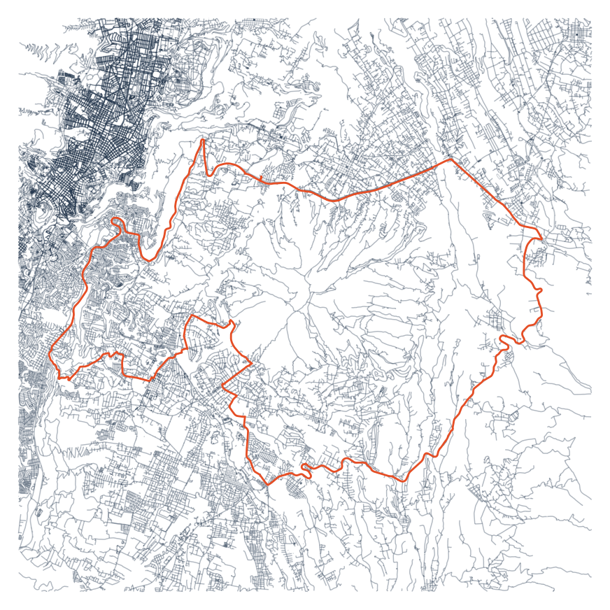

# save figure
fig.savefig('activity.png')

4. Plot Elevation

elevation = route_df.elevation
x_plot    = range(len(elevation))
min_elev  = min(elevation) - 25

# Set the figure size
fig, ax = plt.subplots(figsize=(11, 2))
# Area plot
ax.fill_between(x_plot, elevation, color="#E64E25")
# Set the minimum and maximum values for the y-axis
ax.set_ylim(min_elev, 4000)
plt.axis('off')
# Save the figure
path_save = path.split(".")[0] +"_elevation" ".png"
plt.savefig(path_save , transparent=True, bbox_inches='tight', pad_inches=0 )
# Display the plot
plt.show()

fig.savefig('perfil.png')